Theory of Production
In this lecture, we’ll survey some ideas from the theory of production. The purpose of this theory is to understand how firms make production decisions. This includes the decision of how many of each input factor to employ (i.e. labor and capital) and how much output to produce. The ideas from this lecture are often used in macroeconomic models that try to explain factor prices like wages and interest rates.
General Setup
A firm has a production process that uses labor and capital. Labor refers to human effort, whereas capital refers to things like equipment, machines, land, and software. If the firm employs \(L\) units of labor and \(K\) units of capital, it produces \(Y\) units of commodity output. The relationship between output \(Y\) and inputs \(L\) and \(K\) is given the production function, \(f(L,K)\):
\[Y = f(L,K)\]The firm is a price taker in both the commodity market and the factor markets. It can sell its output commodity at unit price \(p\), it employs labor at unit wage rate \(w\), and it employs capital at unit price \(r\).
The firm’s optimization problem is therefore:
\[\max_{L,K} ~ pf(L,K) - wL - rK\]That is, the firm chooses how much labor \(L\) and capital \(K\) to employ in order to maximize its profits.
First order conditions
The first order conditions for a maximum are:
\[\begin{align} pf_L(L, K) - w = 0 \\ pf_K(L, K) - r = 0 \end{align}\]which can be rearranged to:
\[\begin{align} w = pf_L(L, K) ~ ~ ~ ~ (1) \\ r = pf_K(L, K) ~ ~ ~ ~ (2) \end{align}\]Equation (1) says that at the firm’s optimum, the wage rate is equal to the marginal revenue product of labor. Equation (2) says that at the firm’s optimum, the price of capital is equal to the marginal revenue product of capital. These relations should be familiar to us by now.
If we divide equations (1) and (2), we get:
\[\frac{ f_L (L, K) }{ f_K (L, K) } = \frac{w}{r} ~ ~ ~ ~ (3)\]The left hand side of equation (3) is the ratio of the marginal product of labor to the marginal product of capital. We call that the marginal rate of technical substitution.
Definition
The marginal rate of technical substitution (or MRTS) between two factor inputs is the ratio of the marginal product of those two inputs.
Equation (3) says that at the firm’s optimum, the marginal rate of technical substitution between labor and capital must equal the ratio of the wage rate to the price of capital.
Intuitively, you can think of it like this: the MRTS is the rate at which the firm can substitute labor for capital in its own production process while keeping the same amount of output. The ratio of wage to capital price is the rate at which the firm can substitute labor for capital in the market. If the two do not match, then the firm can produce the same amount of output at lower cost, i.e.
- If the wage rate is too high relative to the price of capital, the firm hires less labor and deploys more capital while maintaining output, thus lowering costs.
- If the wage rate is too low relative to the price of capital, the firms hires more labor and deploys less capital while maintaining output, thus lowering costs.
Thus, the firm’s optimum is achieved only when the two ratios are equal.
Economic Insight
Firm behavior implies that in any economic equilibrium, the ratio of any two factor input prices must equal the marginal rate of technical substitution between those two factors.
Returns to Scale
An important aspect of the production function is its returns to scale. “Returns to scale” asks the question: if all inputs are scaled up or down by an equal factor, how does that affect the commodity output?
- If scaling all inputs up or down by \(X\%\) results in a \(X\%\) change in output, then we say that the production function has constant returns to scale.
- If scaling all inputs up or down by \(X\%\) results in a smaller than \(X\%\) change in output, then we say that the production function has decreasing returns to scale.
- If scaling all inputs up or down by \(X\%\) results in a larger than \(X\%\) change in output, then we say that the production function has increasing returns to scale.
Example
A firm increases its labor and capital inputs by 10%. Its output increases by 8%. Does the firm has constant, increasing, or decreasing returns to scale?
Answer. Decreasing returns to scale.
Example
A firm decreases its labor and capital inputs by 5%. Its output decreases by 10%. Does the firm has constant, increasing, or decreasing returns to scale?
Answer. Increasing returns to scale.
Example
A firm increases its labor and capital inputs by 7%. Its output increases by 7%. Does the firm has constant, increasing, or decreasing returns to scale?
Answer. Constant returns to scale.
Example
A firm increases its labor input by 8% and its capital input by 3%. Its output increases by 5%. Does the firm has constant, increasing, or decreasing returns to scale?
Answer. Unknown. The definition of returns to scale only applies when both inputs are scaled up or down by equal amounts.
Why is the concept of returns to scale important? It closely relates to the average total cost curve (ATC) you might have learned in your Microeconomic Principles classes.
- If a firm’s production function has increasing returns to scale, its average total cost is decreasing in output, and we say it has economies of scale.
- If a firm’s production function has decreasing reurns to scale, its average total cost is increasing in output, and we say it has diseconomies of scale.
- If a firm’s production function has constant returns to scale, its average total cost and its marginal cost curve is constant, which implies an elastic supply curve.
Whether a firm’s production function exhibits constant, increasing, or decreasing returns to scale therefore has important implications for its economic performance and on the
Cobb Douglas Production Functions
A commonly used model of the production function is the Cobb Douglas production function. A Cobb Douglas production function has the following form:
\[f(L,K) = AL^{a} K^{b}\]The Cobb Douglas production function is governed by three parameters, \(A\), \(a\), and \(b\):
- \(A\), called the total factor productivity, controls how productive the firm is overall.
- \(a\) controls the relative importance of labor in the production process.
- \(b\) controls the relative importance of capital in the production process.
An interesting feature of the Cobb Douglas production function is that you can tell whether it has constant, increasing, or decreasing returns to scale simply by looking at \(a\) and \(b\).
- If \(a + b = 1\), then the Cobb Douglas production function has constant returns to scale.
- If \(a + b < 1\), then the Cobb Douglas production function has decreasing returns to scale.
- If \(a + b > 1\), then the Cobb Douglas production function has increasing returns to scale.
Proof
Suppose both \(K\) and \(L\) are scaled by a factor of \(\alpha>1\).
\[\begin{align} f(\alpha L, \alpha K) &= A(\alpha L)^{a} (\alpha K)^{b} \\ &= A \alpha^a L^a \alpha^b K^b \\ &= \alpha^{a+b} A L^a K^b \\ &= \alpha^{a+b} f(L, K) \end{align}\]
- If \(a+b=1\), then \(f(\alpha L, \alpha K) = \alpha f(L, K)\). That is, the production is scaled by exactly \(\alpha\), so the firm has constant returns to scale.
- If \(a+b<1\), then \(f(\alpha L, \alpha K) < \alpha f(L, K)\), so production is scaled by less than \(\alpha\), and the firm has decreasing returns to scale.
- If \(a+b>1\), then \(f(\alpha L, \alpha K) > \alpha f(L, K)\), so production is scaled by more than \(\alpha\), and the firm has increasing returns to scale.
Example
A firm uses labor \(L\) and capital \(K\) to produce a commodity output. The production function is:
\[f(L, K) = L^{1/2} K^{1/4}\]Does the firm exhibit increasing, decreasing, or constant returns to scale?
Answer.
Since \(a = 1/2\) and \(b = 1/4\), \(a + b = 3/4 < 1\), so the firm has decreasing returns to scale.
Cost Minimization
A useful, alternative formulation to the profit maximization problem is the cost minimization problem. The cost minimization problem is especially useful when analyzing firms that have constant returns to scale. The idea behind cost minimization is to ask: what is the minimum cost for me to produce 1 unit of output?
The cost minimization problem is written as follows:
\[\min_{L, K} ~ wL + rK ~ \text{ s.t. } ~ f(L,K) = 1\]That is, choose \(L\) and \(K\) to minimize cost, such that the total amount of output is 1 unit.
First order conditions
This is a standard contrained multivariate optimization problem. The first order conditions are:
\[\begin{align} w &= \lambda f_L(L, K) \\ r &= \lambda f_K(L, K) \end{align}\]The two first order conditions and the constraint \(f(L,K)=1\) gives us three equations in three unknowns: \(L\), \(K\), and \(\lambda\). The system can thus be solved for the optimal combination of labor and capital to use to produce one unit of output, as well as the cost to produce one unit.
Example
A firm has a constant returns to scale production function over labor and capital given by:
\[f(L, K) = \frac{1}{4} L^{3/4} K^{1/4}\]The unit price of labor is \(w=5\) and the unit price of capital is \(r=4\).
- What choice of labor minimizes the cost to produce one unit of output?
- What choice of capital minimizes the cost to produce one unit of output?
- What is the firm’s cost to produce one unit?
Answer.
Step 1. Write down the cost minimization problem.
\[\min_{L, K} ~ 5L + 4K ~ \text{ s.t. } ~ \frac{1}{4} L^{3/4} K^{1/4} = 1\]Step 2. Write down the first order conditions.
\[\begin{align} 5 &= \frac{3}{16} \lambda L^{-1/4} K^{1/4} \\ 4 &= \frac{1}{16} \lambda L^{3/4} K^{-3/4} \end{align}\]Step 3. Divide the two first order conditions and simplify.
\[\begin{align} \frac{5}{4} &= \frac{3 L^{-1/4} K^{1/4}}{L^{3/4} K^{-3/4}} \\ \frac{5}{4} &= \frac{3 K}{L} \\ L &= \frac{12}{5} K \end{align}\]Step 4. Plug \(L = \frac{12}{5}K\) into the constraint and solve for \(K\).
\[\begin{align} \frac{1}{4} L^{3/4} K^{1/4} &= 1 \\ \frac{1}{4} \left( \frac{12}{5} K \right)^{3/4} K^{1/4} &= 1 \\ \frac{1}{4} \left( \frac{12}{5} \right)^{3/4} K^{3/4} K^{1/4} &= 1 \\ \frac{1}{4} \left( \frac{12}{5} \right)^{3/4} K &= 1 \\ 0.4821 K &= 1 \\ K &= 2.0744 \end{align}\]Step 5. Plug \(K=2.0744\) into \(L = \frac{12}{5}K\) to get \(L\).
\[L = 4.9787\]Step 6. Plug \(L\) and \(K\) into the \(5L + 4K\) to get the cost to produce 1 unit.
\[MC = 5 \times 4.9787 + 4 \times 2.0744 = 33.191\]
Graphical representation of cost minimization
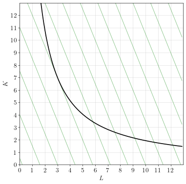
Cost minimization can be represented graphically by an isoquant and isocost curves, as illustrated below.
The curved black line is called an isoquant. It represents the combinations of \(L\) and \(K\) that can be combined to produce one unit of output. It is our constraint in the cost minimization problem.
The straight green lines are called isocost curves. Think of these as contour lines representing a hill, and the hill is the total cost for employing different combinations of labor and capital. The hill is rising in the northeast direction, but our goal is to minimize costs, not to maximize them.
The choice of \(L\) and \(K\) that minimizes costs is the lowest point on the hill that’s touching the constraint. That occurs when the isocost curves are tangent to the isoquant: \(L=5\) and \(K=5\).
Example
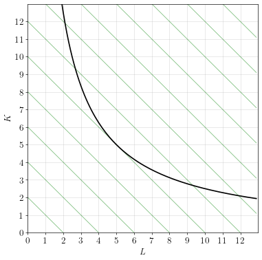
A firm has a constant returns to scale production function. Its unit isoquant and isocost curves are shown in the diagram below.
The unit price of labor is \(w=5\) and the unit price of capital is \(r=2\).
- What choice of \(L\) and \(K\) minimize the cost to produce one unit?
- What is the cost to produce one unit of output?
Answer.
The cost to produce one unit is minimized when \(L=3\), \(K=7\). The cost to produce one unit is \(5 \times 3 + 2 \times 7 = 29\).